You can calculate the savings from a lighting control system in three steps. First, determine the current electricity consumption of the lighting from the installed load and operating hours. Next, set a realistic reduction factor for each control function (occupancy, daylight, constant light output) and combine them multiplicatively, not additively. Finally, deduct the standby consumption of the sensors, value the kilowatt hours saved at your electricity price and compare the result with the investment. This guide sets out the formulas, a fully worked example and the typical mistakes that distort cost-effectiveness calculations.
Step 1: Determine the baseline consumption
Every calculation starts with the consumption without controls, known as the baseline consumption:
E_ref = P_inst × t_op
- P_inst: installed electrical load of the lighting in kW (sum of luminaire wattages including control gear)
- t_op: annual operating hours without controls in h/year
You can determine the installed load from the luminaire schedule or a site survey. Do not derive the operating hours from core working hours, but from the actual time the lights are on: in many buildings, the lights are on from the moment the first employee arrives until the cleaners leave in the evening. Where measurements or meter data are available, they are always better than estimates.
Step 2: Reduction factors for the control functions
A modern lighting control system combines several functions. Each one reduces consumption by a certain proportion:
- Occupancy control (f_P): The lights are only on or dimmed when the area is in use. The basics are covered in our article on presence detectors vs. motion detectors.
- Daylight harvesting (f_D): Artificial lighting is dimmed according to the amount of incoming daylight. Details in daylight harvesting.
- Constant light output / task tuning (f_C): New installations are oversized to allow for the maintenance factor; regulating to the level actually required saves this reserve.
Why you have to multiply
The functions act one after another on the same consumption. Daylight control only saves energy during the hours when the lights are switched on because the space is occupied. The formula is therefore:
E_new = E_ref × (1 − f_P) × (1 − f_D) × (1 − f_C)
If you simply add the factors together (30 % + 25 % + 10 % = 65 %), you overestimate the savings. With these values, the correct total saving is 52.75 %.
Guideline values for the factors
The following ranges are typical guideline values for preliminary planning. They depend heavily on usage, façade, time delays and the starting point, and are no substitute for measurement.
| Function | Area | Typical range (guideline) |
|---|---|---|
| Occupancy | Private and shared offices | 20–40 % |
| Occupancy | Corridors, stairwells, ancillary rooms | 30–60 % |
| Occupancy | Low-traffic warehouses | 40–70 % |
| Daylight | Window zone | 20–40 % |
| Daylight | Interior zone without rooflights | 0–10 % |
| Constant light output | New LED installation | 5–15 % |
In combination – especially in rarely used areas and warehouses with rooflights – savings of up to 90–92 % are possible with occupancy and daylight control at luminaire level. For normal office use, you should calculate more conservatively.
Step 3: Deduct the sensors' own consumption
Sensors and wireless modules are in operation around the clock. Their own consumption is low, but it belongs in any sound calculation:
E_self = n_devices × P_device × 8,760 h
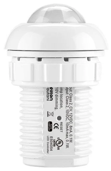
You will find the power consumption in the datasheet. For example, a maximum of 0.3 W is specified for the IFS105SE sensor and 0.5 W for the FA102 Bluetooth node. Battery-powered sensors such as the BCS107 draw no mains power, but the battery needs replacing after a number of years.
The net saving is then:
ΔE = E_ref − E_new − E_self
Step 4: Costs, payback and net present value
The annual cost saving is calculated as:
C_saving = ΔE × electricity price
The simple payback period is the most straightforward metric:
T_payback = investment / C_saving
More meaningful is the net present value (NPV), which takes the cost of capital into account:
NPV = −investment + C_saving × PVAF(i, n) with PVAF = (1 − (1 + i)^−n) / i
Here, i is the discount rate and n the evaluation period in years. PVAF is the present value annuity factor.
Worked example: 1,000 m² office floor
Important: all values are example assumptions to illustrate the calculation method. Use your own values for your project or try the savings calculator.
Starting point: a 1,000 m² office floor is already fitted with LED luminaires (7 W/m², 120 luminaires). The lights are currently on for around 2,750 hours a year. The plan is to retrofit 120 luminaire-level sensors, each with a power consumption of 0.3 W.
| Calculation step | Formula | Example value |
|---|---|---|
| Installed load | 1,000 m² × 7 W/m² | 7.0 kW |
| Baseline consumption | 7.0 kW × 2,750 h | 19,250 kWh/year |
| Occupancy control | f_P (assumption) | 30 % |
| Daylight harvesting | f_D (assumption) | 25 % |
| Constant light output | f_C (assumption) | 10 % |
| Residual factor | 0.70 × 0.75 × 0.90 | 0.4725 |
| Consumption with controls | 19,250 × 0.4725 | 9,096 kWh/year |
| Gross saving | 19,250 − 9,096 | 10,154 kWh/year (52.75 %) |
| Sensors' own consumption | 120 × 0.3 W × 8,760 h | 315 kWh/year |
| Net saving | 10,154 − 315 | 9,839 kWh/year |
| Cost saving | 9,839 kWh × €0.25/kWh | €2,460/year |
| Investment (assumption) | Hardware, installation, commissioning | €13,000 |
| Simple payback | €13,000 / €2,460/year | around 5.3 years |
| Net present value after 7 years | −€13,000 + €2,460 × 5.786 (i = 5 %) | around +€1,230 |
The net present value is positive after seven years. Assuming a service life of 14 years, for example, the criterion of a "positive net present value after 50 % of the service life" would be met in this example.
Sensitivity: the effect of the electricity price
The electricity price has a major influence on payback. With the example assumptions otherwise unchanged:
| Electricity price | Annual cost saving | Simple payback |
|---|---|---|
| €0.20/kWh | €1,968 | around 6.6 years |
| €0.25/kWh | €2,460 | around 5.3 years |
| €0.30/kWh | €2,952 | around 4.4 years |
Applying this to warehouses and halls
In warehouses and industrial halls, the picture usually shifts in favour of controls: luminaires have high individual wattages, operating hours are often long because of shift work, and many aisles see only occasional traffic. As a result, the occupancy factor rises significantly. In this case, calculate separately by zone – for example picking, racking aisles and traffic routes – and use separate factors for each zone. You will find advice on choosing sensors for high mounting heights in our guide to high bay sensors for warehouses.
What the calculation often leaves out
Besides electricity, other factors influence cost-effectiveness:
- Luminaire service life: LED luminaires that are dimmed and switched off when not needed reach their rated life later. Maintenance and replacement intervals are extended.
- Cooling load: Less heat from lighting reduces the cooling load in air-conditioned buildings.
- Electrical work saved: Wireless systems do away with control cables. This significantly reduces the investment in existing buildings – see retrofitting lighting controls.
- Use of data: Occupancy and energy data enable space optimisation and predictive maintenance. Find out more in our guide to energy monitoring and occupancy data.
Verifying savings after installation
You should check the calculated savings in operation. With the CR01-ETC energy monitoring dongle, the energy consumption data of a Keilton+autani zone is recorded every 15 minutes as a raw log and analysed for usage reports. At building level, the AU-Manager displays real-time and historical consumption data graphically and stores system events for more than a year. This turns the forecast into a verified figure that you can use for energy audits, implementation plans or ESG reports.
Conclusion
The savings from a lighting control system can be estimated reliably with just a few formulas: baseline consumption from load and operating hours, multiplicatively combined reduction factors, deduction of the sensors' own consumption and valuation at the electricity price. In the example, an office floor saves around 53 % of its lighting electricity and pays for itself in just over five years. Realistic operating hours and conservative factors are essential for robust results. Work through your own scenario with the savings calculator or get advice via our contact page.
Try it interactively
Savings calculator
Frequently asked questions
How much energy does a lighting control system save?
That depends on usage, the proportion of daylight and the starting point. In offices, around 40 to 60 % is often realistic, depending on the combination of occupancy, daylight and constant light control. In rarely used areas and warehouses with rooflights, up to 90–92 % is possible.
Why shouldn't savings factors be added together?
The functions act one after another on the same consumption. Daylight control only saves energy during hours when the lights are on because the space is occupied. The residual factors are therefore multiplied: 30 %, 25 % and 10 % together give 52.75 %, not 65 %.
How many years does it take for lighting control to pay for itself?
The payback period is the investment divided by the annual cost saving. In the example in this guide, it is around 5.3 years at €0.25/kWh. Higher electricity prices, long operating hours and avoiding cabling costs shorten it.
Does the sensors' electricity consumption need to be taken into account?
Yes. Sensors and wireless modules operate continuously. Their consumption is calculated from the number of devices, the power consumption stated in the datasheet and 8,760 hours per year. It is usually small compared with the saving, but belongs in any sound calculation.
How do I verify the actual savings?
With energy monitoring. The CR01-ETC records a zone's consumption data every 15 minutes, and the AU-Manager displays real-time and historical data graphically. This allows you to compare the forecast with actual values.